By Armando Rodriguez
This trend tool takes a date, a pair and a period and delivers a slope for the
ask (quotes) regression and the minimum holding time. The period has following
fixed choices: year, month, week, day and hour.
As the period increases, the number of samples to process also increases. In the
average, there are about 50 quotes every minute for each pair, adding up to
roughly 26 million in a year. This is way more than it is needed for a linear
regression, the tool will keep the sample count below 100000. So, for hourly and
daily periods, all the quotes will be processed; for weekly periods one of every
five; for monthly, one for every 21 and for yearly periods one every 262.
The actual skipping factor is calculated as:
Skip = totalQuoteCount/100000
Only those quotes being issued in the seconds that are integer multiples of the
skip will be processed.
For calculating the regression estimators, the following averages over the
selected samples must be calculated
avgT average of the times within the period
avgT2 average square time within the period
avgQ average of the quotes
avgTQ average of the products of the quote and its time
According to the linear regression formula, the slope S is:
S = (avgTQ - avgT*avgQ)/( avgT2 – (avgT)2)
The intercept I :
I = avgQ – slope*avgT
The equation for the regression line is:
Q(t) = S*t + I
The randomness about the regression line must now be estimated. This uncertainty
(U) can be represented by the square root of the average of the squares of the
residuals, which, assuming normality of the distribution, the standard deviation
of the quotes from the perfect linear behavior. A residual is the difference
between the actual quote and the regression line so:
U = Sn=1toN
(Qn – (S*tn + I))2/N
Considering that the random part of the quotes motions is a Markov Chain, the
next element in the sequence only depends on the present one, so any forecast
must start from the last quote and the trend must show as:
q(t) = q(0) + S*t
From that moment on, still assuming normality, the probability of finding the
quotes away from that last quote will follow a Gaussian function . This Gaussian
broadens into the future with the square root of time. If the randomness stays
the same, the standard deviation (u(t)) must reach the same value as U in the
same period T (hour, day, week, etc.).
u(t) = (U/ÖT)
*Ö
t
The probability of getting a quote within the interval of +/- the standard
deviation around the trend line is about 68%, that of getting one within twice
the standard deviation is 95%. Using this last interval of confidence, the
upper limit (B(t)) or best case scenario for a buy as a function of time will
be:
B(t) = q(t) +2* u(t) = q(0) + (S*t) + (2*U/ÖT)
*Ö
t
The lower limit of the 95% confidence interval (W(t)) or worst case scenario for
a buy, will then be:
W(t) = q(t) - 2*u(t) = q(0) + (S*t) - (2*U/ÖT)
*Ö
t
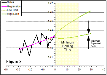
For small values of t, W(t) will less than q(0), meaning that, for a buy,
there’s a chance within the confidence interval for a loss. In other words, the
time is too short for the trend to reveal over the randomness. There is a
minimum time that a position must be held for the whole interval of confidence
to go above the initial quote. Calling this the minimum holding time or MHT:
MHT = 4*U2/(T*S2)
A sell scenario would involve a negative trend and then the worst case would be
the upper limit. A plot of the forecast consists of an inclined parabola ant the
MHT would be the intercept with the last quote level.