Transmitter Calibration Procedure
Beside the fact that
there's a complex #include DSP application at the center of the
instrument being calibrated, this calibration procedure
shows expertise in:
- RF Network math.
- TCAS technology
- RF instrumentation
- Measurement
automation (GPIB)
- National
Instruments CVI programming
- Technical
Documentation
Connecting the instrument and Special Tools
These calibrations require
a Network Analyzer, NA hereafter, featuring a GPIB interface like the E5062A by
Agilent Technologies. This instrument must be calibrated before attempting any
of the procedures below.
Make a “Thru
Calibration S21” in the NA, observe using the same cable to be attached to “
Port 1” during the measurements when calibrating.
Special Tool #1 is a cable that has been cut to guarantee that its attenuation,
plus the one from the UUC (Unit Under Calibration) CAL input to the
Synthesizer-to-CAL internal switch adds up to exactly 2dB.
Connect Special Tool
#1 from the NA’s Port 2 to the UUC CAL input.
Figure 9.9
Charlotte, Special Tool #2
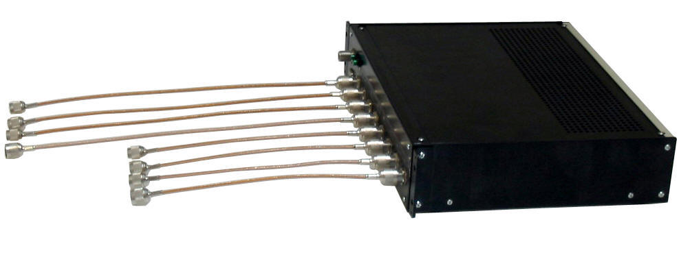 Special
Tool #2 is a RS-232 controllable 1-to-8
RF MUX. It was named Charlotte, for its resemblance to a spider in its
original version, after the famous
Hanna-Barbera character.
Charlotte (present
look shown in Figure 9.9)
must connect to the RF female connectors T1 through B4 out the UUC front panel;
the RS-232 DB9 to the host computer and its RF output to the NA’s RF-IN (Port
1).
Special
Tool #2 is a RS-232 controllable 1-to-8
RF MUX. It was named Charlotte, for its resemblance to a spider in its
original version, after the famous
Hanna-Barbera character.
Charlotte (present
look shown in Figure 9.9)
must connect to the RF female connectors T1 through B4 out the UUC front panel;
the RS-232 DB9 to the host computer and its RF output to the NA’s RF-IN (Port
1).
Other connections are: UUC CAL input connects to the NA’s RF-OUT; REF OUT
connects to the BNC at the back of the NA labeled Ext. Ref In; GPIB connector on
the Network Analyzer to the GPIB on the host’s GPIB board and the USB connector
from the host to the UUC.
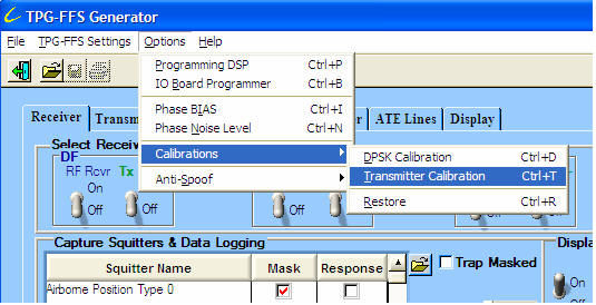
Select the Transmitter Calibration item under Option/Calibrations as shown in
Figure 9.10. Upon selection, you will be prompted for a password. Next, there
will be a prompt for the GPIB device address of the instrument:
|
Selecting the menu item |
|
Figure 9-10 |
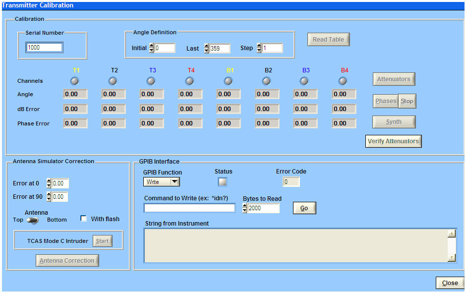
Finally the Transmitter
Calibration window opens. The upper half of the windows shows the Calibration
Frame with everything relating to the calibration procedures at hand.
|
Transmitter Calibration Window |
|
Figure 9-11 |
At the lower right, there
is the GPIB frame for issuing direct GPIB commands to the instrument (this is
only useful for troubleshooting). On the left-bottom corner you find the frame
for introducing the antenna simulator correction, which is done after finishing
all the calibrations and does not require the Network analyzer or Charlotte, but
must be connected to a TCAS.
Figure 9.11 shows that
most of the buttons on the window are dimmed; this is because the mode shown is
that of the phase settings calibration. During this process, that can take up to
90 minutes, you are only allowed to abort by hitting the Stop button.
If the unit has never been
calibrated before, the Serial Number on the top left corner will show as 1000,
otherwise the current unit serial number will have already been read and
displayed. In
case of a first time calibration or if the serial number need to be changed, the
first step must be entering the serial number for the unit.
The signals from UUC may
be set to power levels varying from -20 dB to -90 dB +/-.5 dB in 1 dB steps.
This is accomplished by four 96 dB digital adjustable attenuators, one for each
channel.
Each one of these 96 dB
att’s, is built using a series of three 32 dB att’s. Since there is a phase
shift introduced by these attenuators that may vary with the attenuation
selected, there must be a table that stores a phase correction for each of the
70 selectable attenuation values. Also there’s a code to be set to these
attenuators to obtain the desired attenuation, meaning there must be a table
storing these codes to actually obtain de desired value at the UUC output.
The phase shifts can grow
to be as much as 7 degrees for some codes, but the difference from one
attenuator to another having applied the same code was measured to be less than
0.5 degrees. Since it is only the difference what counts, if all the att’s had
the same codes, the correction would be smallest. To take advantage of this,
there’s a hurdle to overcome and it is that the channel/antenna path attenuation
is different for every channel. To solve the issue, these differences will be
compensated using only the first of the 3 attenuators and this is what present
adjustment is about. The phase differences for not having the same codes would
get compensated together with the rest of the effects when creating the phase
tables in the next adjustment. When testing for different power levels, the
first 60 operational dB’s will be set by using the same codes on the other two
for all the channels, thus introducing only the mentioned minimum deviations.
Beyond 60 dB, the phase becomes irrelevant for the UUC specifications, so these
attenuations can be coded freely into the first attenuator disregarding any
phase shifts that could arise from the difference in codes.
The goal of this
adjustment is to get -19.5 dB on each channel by adjusting the first attenuator
while the other two remain in 0 dB. The IQ’s vary from -2047 to +2047, for this
adjustment they are set as follows:
I1 = 877;
Q1 = 1687;
I2 = 1900;
Q2 = 0;
I3 = 877;
Q3 = -1687;
I4 = 1900;
Q4 = 0;
This is consistent with a
radius of 1900 and zero airplane angle. A 247 margin to it maximum value will
allow up to a 10% correction of the output signal level with the values of IQ.
To execute the adjustment, just hit the Attenuators button in the Calibration
frame. The dB error can be followed as it converges to zero, one channel after
another. The LED activity indicator on top of the channel being adjusted will
lit in green.
The purpose to the UUC
tables is to create for the TCAS the right signals to simulate the ones that
would come from an intruder plane in a given position. These signals must have
relative phases consistent with the bearing of such an intruder.
Theoretical phase
differences respond to the following equations:
Being element 0 the one
nearest to the front of the plane for the top antenna we have:
P01 = (2P
L/ l)
(cos B + sin B)
P11 = 0
P21 = -(2P
L/ l)
(cos B + sin B)
P31 = -2(2P L/
l) sin B
But these phases are not
the ones actually measured, because of the different in paths leading to the
connectors. Also, the channel circuits are not perfectly isolated, thus allowing
the signal in one channel to affect the phase of the signal in the others. So,
the actual phase must be corrected in a value that is a function of the antenna
being top or bottom, the channel and the airplane angle. To introduce this phase
correction a STQ-2016 quadrature modulator is used for each channel. The way it
works is that, for every angle (in one degree increments), the 360 values of I
and the 360 values of Q for each channel and for each antenna must be looked up
a total of eight tables. The purpose of this process is to obtain these tables.
To start the process hit the Phases button.
Starting with the “Initial” airplane angle, it will recur through all the
channels until has attained the correct values of I and Q to render the right
phase and amplitude. Then it will increment this angle in the “Step” value, and
repeat the process all the way to the “Last”. On the Network Analyzer screen,
which is set to Polar display, the phasor will be seen jumping from one point in
the -20dB circumference to another as Charlotte switches the channels. Each
angle takes about 12 to 15 seconds.
The whole process
takes about 90 minutes.
By default the process
will go through all the angles from 0 to 359, but it requiring so much time, a
smaller range could be chosen in case that, for instance, it happens to be the
continuation of a preceding partial process. When it’s done the table will be
flashed and an image of the tables and saved to a file named IQXXXX.dat, where
XXXX is the UUC serial number.
In order to make
calibration deviation estimate, the values of phase and amplitude before and
after are recorded into the following files respectively:
phInitXXXX.dat
phFinalXXXX.dat
dBInitXXXX.dat
dBFinalXXXX.dat
Warning:
Since the IQ values can not correct the signal level variations beyond
10%, the attenuator adjustment process should precede this one.
This adjustment should be
the last one to be performed, this will guarantee that the 0 dBm provided by the
network analyzer at the Cal/Synth switch input will render -20 dB output. Now
the synthesizer level must be adjusted to deliver the same 0 dBm for 1030 MHz as
well as for 1090 MHz.
The user interface will
set the Network analyzer to external reference, this external reference is
connected, as said above, to the REF OUT. The power will then be measured and a
corresponding increment sent to the DSP via CmdID 69 ordering the DSP to send an
increment command through the SPI link to the potentiometers AD5232. The process
will iterate until the -20 +/-0.5 dBm is read at the T1 output. While this is
happening, the Network Analyzer should show what looks like a yarn ball that
expands or contracts until the outer radius reads -20 dBm.
The potentiometer wiper is
saved every time CmdID 69 command is issued and the calibration value set to the
voltage being read from the DSP internal ADC. CmdID 69 does not flash these
results, so CmdID 37 is issued after the correct levels have been attained.
When it’s done the values obtained together with other miscellaneous setting
will be flashed and saved to a file named miscXXXX.dat, , where XXXX is the UUC
serial number.
To execute this adjustment, just hit the button “Synth”.
Verify Attenuators
The purpose of this
process is to verify that the attenuation between -20 and -50 dB is within 1dB
and that between 51 and 80 dB is within 3 dB. As the verification progresses the
deviations are shown on the db Error text boxes. The first 8 values found out of
range will pop up a message box; hitting OK the process will continue. There’s
no adjustment to be made, it is a true or false thing. A unit not meeting these
requirements must be repaired.
To execute, hit Verify
Attenuators.
When TCAS is transmitting
to the UUC it is the antenna simulator that absorbs the power. TCAS will
calibrate periodically, this is, it will update the compensating phase
difference in the RF paths by comparing the phases P12 to P32 when irradiating
from 2 and similarly, somehow, it also
finds a correction for P42. With a perfect antenna simulator this wouldn’t pose
a problem, since it wouldn’t add any phase shift to the one introduced to the
external cables and connectors.
Unfortunately, it is not perfect and TCAS will compensate for its asymmetries.
Typical errors introduced by asymmetries in the antenna simulator are shown in
Figure 9-12
To determine the TCAS correction, four static
Mode C intruders are generated with bearings of 0, 90, 180 and 270 degrees. TCAS
will see different bearing values due to the mentioned correction. From these
differences in bearing the actual phase corrections can be calculated and thus
compensated.
Intruders are generated by hitting the Start
button. TCAS is then allowed to compensate these bearings so that the errors can
be recorded. Bearing deviations for 0 and 180 are averaged (DB0),
then the same for +/-90 degrees (DB90).
DB0
and DB90
should be keyed into the text boxes Error
at 0 and Error at 90 respectively; then the Antenna
Correction button must be hit to finish the entry.
The correction can be considered compensated
when the readings for DB0
and DB90
show smaller than 0.5
degrees, only then is that the correction
parameters should be flashed. This is done by checking the With Flash
box then hitting Antenna Correction again. This procedure must be
performed for both Top and Bottom antennas. Antenna selection is done with the
Antenna switch.
Math for the compensation of TCAS correction to the antenna simulator
Let
K be:
K = 2P L/l
(1)
Then the phases as relate to the intruder bearing as;
f12
= K(cos(B) - sin(B)) (2)
f32
=-K(cos(B) + sin(B)) (3)
f42
=-2Ksin(B) (4)
Or that B relates to the phases as:
B = cos-1((f12
- f32)/2K)
(5)
B =-sin-1((f12
+ f32)/2K)
(6)
B =-sin-1(f42
/2K) (7)
Now assume that the paths conveying the signals
to the phase detector introduce phase differences of df12,
df32 and df42.
We will assume these to small as to approximate the sine to the angle.
For B = 0, these phase differences will introduce the
effect of deviating the reading in DB.
If calculated from (7):
DB0
=-df42/2K
(8)
Differentiating in (5) and evaluating at
P/2:
DB90
= (df12 - df32)/2K
(9)
But from (6):
(f12 +
f32)/2K
=-sin(B)
(10)
Differentiating:
(df12 + df32)/2K
=-cos(B)dB (11)
For B = P/2,
cos(B) = 0, then:
df12 = -df32
(12)
Combining (8), (9) and (12)
df42 = 2DB0K
(13)
df12 = -df32
= DB90
K
(14)
For the bottom antenna, the reference becomes 4 instead
of 2, then:
df24 = -2DB0K
(15)
df14 = -df34
= DB90
K
(16)
Now, our antenna simulator is introducing these small
path differences when TCAS is calibrating. TCAS calibration will compensate for
all path differences, including paths internal to TCAS as well as external ones,
like cable, connectors and the antenna simulator’s asymmetries. Our transmitter
inserts its signal into these paths with no phase differences (UUC airplane
bearing angle to phase tables were calibrated to that condition), the TCAS
compensation will work except for the mentioned antenna simulator’s asymmetries
that can only be seen from TCAS.