Simulating aircraft motion is currently used for many purposes. In this case we need to simulate an aircraft that must fly through a set of waypoints in a realistic manner. By realistic it is meant that broken line trajectories are not acceptable and that turn radiuses must be considered.
Climbs and descends further complicate the problem because, in principle, the speed is no longer a “cruise” speed. While in a climb, aircrafts normally slow down and when combined with a turn, the banking angle must be substantially reduced. Even though the increase in distance due to an altitude difference is normally negligible (the first goes in nautical miles and the second in feet), calculation of the flight time may become tricky for nearby waypoints. Also, combined maneuvers raise a lot of options. A climb, for instance, may take less time than a turn, so the climb may be slowed down to match the turn; the climb can be done at the beginning of the turn, at the end, or even completely after the turn during the straight flight. For a simulator to take an optimum choice, the aircraft must be characterized with additional parameters, like power and cargo load which are currently not handled by the simulator.
The policy here will be that the “reality” of simulating waypoints at different altitudes will be transferred to the scenario designer. The simulator will operate as follows:
When a position waypoint is in effect, the m_g[] floating point parameters of waypoints type 3 will have a different interpretation:
Type 3 Way Point
m_g[0] Banking angle, in degrees
m_g[1] Cruising speed, in knots
m_g[2] Max Vertical Rate, in feet per minute.
· Vertical motion will superimpose to the simulated aircraft motion in the XY plane, which increases the resultant speed.
· Vertical rate will come into effect right after a waypoint type 3 sets it to a value different than zero.
· The altitude will start changing at the specified rate until it matches that of the next position way point, at which point the vertical rate will be set back to zero.
· When a position waypoint is over flown, it will no longer be in effect. When this happens last course will be kept as well as the last altitude.
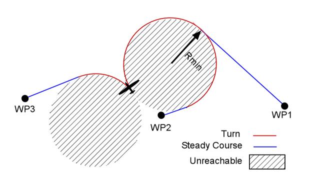
A real aircraft with a real pilot have infinite maneuver choices for flying from one waypoint to the next. For simulation purposes, the trajectory of choice between waypoints of equal altitude will be the one that minimize the flight time, consisting of a turn with maximum banking angle in order to attain a minimum turning radius and then a steady course to the waypoint.
From the above graphic, it is obvious that points within the shaded area are unreachable with the described maneuver, so no waypoints may be specified there.
The problem may be split in two; one part that deals with the calculation of the real flight time between way points and a second part that has to do with the real time trajectory simulation.
This first part is needed for the planning stage of the simulated flight. The simulated aircraft, at its current position, reads the position of the waypoint it must fly to. The simulated aircraft will start turning toward this waypoint until it reaches the right course, then it will keep this course until the waypoint is reached. Precisely at this point, a new waypoint must be read, since waypoints are read at their specified time, the flight time must be known at simulation design time.
In other words, the real-time simulator that runs on its DSP must be provided with a sequence of way points, each of which has a time label. Every 100 ms, this real-time simulator will check if it is time for the next waypoint in line to go active. The next waypoint must go active when the present waypoint is reached (or even before but never after). This means that the fly time between waypoints must be known when creating the waypoint sequence, before the simulation starts.
|
Cruise Speed
Knots |
Turn Radius
(nm) |
Turn rate in
Degrees/s |
|
120 |
0.45 |
4.244132 |
|
140 |
0.6125 |
3.637827 |
|
160 |
0.8 |
3.183099 |
|
180 |
1.0125 |
2.829421 |
|
200 |
1.25 |
2.546479 |
|
220 |
1.5125 |
2.314981 |
|
240 |
1.8 |
2.122066 |
|
260 |
2.1125 |
1.95883 |
|
280 |
2.45 |
1.818914 |
|
300 |
2.8125 |
1.697653 |
|
320 |
3.2 |
1.591549 |
|
340 |
3.6125 |
1.497929 |
|
360 |
4.05 |
1.414711 |
|
380 |
4.5125 |
1.340252 |
|
400 |
5 |
1.27324 |
|
420 |
5.5125 |
1.212609 |
|
440 |
6.05 |
1.15749 |
|
460 |
6.6125 |
1.107165 |
|
480 |
7.2 |
1.061033 |
|
500 |
7.8125 |
1.018592 |
 The
turn radius depends on the cruising speed and the bank angle. This bank angle is
limited by the acceleration that the aircraft can withstand. If you tilt a plane
in a straight flight, it loses its lift and drops, but it you tilt and pull up,
then it turns without dropping. With the right “pull-up”, the inclined lift
force is augmented to the point that its vertical component will compensate its
weight avoiding the drop in altitude. When a turn is done right, gravity inside
the plane is increased while remaining vertical to the floor. You may have
experienced this effect while flying when you see that the liquid in you drink
stays at level even when the aircraft goes into a turn. So again, in a perfect
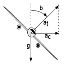
turn, the bank angle determines the acceleration vector. Let
b be the banking angle,
at the total acceleration
and g the acceleration of gravity,
then:
The
turn radius depends on the cruising speed and the bank angle. This bank angle is
limited by the acceleration that the aircraft can withstand. If you tilt a plane
in a straight flight, it loses its lift and drops, but it you tilt and pull up,
then it turns without dropping. With the right “pull-up”, the inclined lift
force is augmented to the point that its vertical component will compensate its
weight avoiding the drop in altitude. When a turn is done right, gravity inside
the plane is increased while remaining vertical to the floor. You may have
experienced this effect while flying when you see that the liquid in you drink
stays at level even when the aircraft goes into a turn. So again, in a perfect
turn, the bank angle determines the acceleration vector. Let
b be the banking angle,
at the total acceleration
and g the acceleration of gravity,
then:
cos b = g/ at eq 1
Then the centripetal acceleration would be.
ac = at sin b eq 2
The turn radius can be then be expressed in terms of the cruise speed Vc and the centripetal acceleration at:
R = Vc2/ac eq 3
Manipulating the above expressions we can get to:
R = Vc2/ Ö(at2 – g2) or
R = (1.4581759 x 10⁻⁵) Vc2/ Ö(at2 – 1) eq 4
That renders R in nautical miles for Vc in knots and at in g’s (gravities). A typical value of at for a passenger aircraft is 1.1 that corresponds to banking angle of 24.6 degrees. To the left, there is a table of radiuses and turning rates for this banking angle.
The trajectories within the simulator CPU are calculated using the earth’s ellipsoid model and ECEF Cartesian coordinates, but for accuracies within a second in flight time and latitudes under the Polar Circle, plane geometry should do the job.
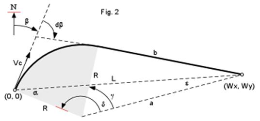
Let’s consider an aircraft with a cruising speed Vc and a heading angle b, that, when flying over (0,0) received a waypoint situated at Wx nm to its East and Wy nm to the North (or South as in the example). The total trajectory length P is the sum of the turning arc plus segment b.
P = Rdb + b eq5
Let L be the distance to the waypoint:
L = Wx + Wy eq6
a is the complement to the initial waypoint bearing:
a = p/2 – (b - atan2(Wx.Wy)) eq7
The cosine law provides an expression for a:
a2 = L2 + R2 + 2RLcos a eq8
Since b, a and R make a triangle rectangle:
b2 = a2 - R2 = L2 + R2 + 2RLcos a eq9
All we need now is db, but for that we are going to need a few angles to get there…
The sine law allows an expression for e:
sin
e
/ R = sin a
/a
eq10
sin
g
= b/a
eq 11
d = p – a – e eq12
Finally:
db = g - d eq13
Expression for the flight time Tf is simple:
Tf = P/Vc eq 14
Where P, from eq 5, is the total trajectory length and Vc the cruising speed. However, the above expressions may become tricky to write into a program. This is because the signs and discontinuity of angles may get complicated when attempting to cover the most general case of any angle and any valid waypoint position. A way to simplify things is to reduce every problem to the above. Since any symmetric trajectory renders the same flight time, there’s no great offense in doing this. The heading angle must be reduced to the top quadrants (+/- 90) and the waypoint to the right quadrants. For heading in the bottom quadrants, the scenario must be reflected on X axis. For waypoints on the left quadrants the reflection must be on the Y axis.
This part runs in the simulator DSP. Trajectories are calculated in an incremental fashion. Time is divided in dt intervals (one second is actually used), when the timer ticks, position, velocity and acceleration vectors will be incremented in accordance with the motion differential equations. Upon a new waypoint becoming active, the intruder will go into a circular motion with angular speed w until it heads to the waypoint.
w = Vc/R eq 15
Where Vc is the cruising speed and R is the turning radius that comes from eq 4. The heading at interval n, H(n), relates to the previous heading as:
H(n) = H(n-1) + dH(n) eq 16
During the turn:
dH = wdt eq 17
At interval n, the aircraft sees the waypoint with bearing angle B(n):
B(n) = H(n-1) - atan2(Wx –
X(n-1), Wy – Y(n-1)) eq
18
Where Wx and Wy are the waypoints coordinates; X(n) and Y(n) are the intruder coordinates at interval n. When the bearing angle becomes smaller than wdt, it is time to limit the turn increment dH to the bearing size. So dH(n):
| (|B(n)| /B(n)) wdt for |B(n)| > wdt
dH(n) = | eq 19
| B(n) for |B(n)| < wdt
(|B(n)| /B(n)) is just the sign if B(n), it is 1 if positive and -1 if negative.
Vx(n) and Vy(n) are the projection of the velocity vector at interval n along the X and Y axis respectively, they can be expressed in terms of the bearing heading angle H(n) as:
Vx(n) = Vc*cos(H(n))
eq 20
Vy(n) = Vc*sin(H(n))
eq 21
Finally we X(n) and Y(n) can relate to their previous values through the velocity sequence. However, if while turning, the present position is incremented with the non-incremented velocity vector, the next point will lie slightly out of the circle. On the other hand, if the incremented velocity vector is used, the next point this time will lie inside the circle. The error drops more than ten times when the half sum of the two velocity vectors is used for incrementing the position:
X(n) = X(n-1) +
((Vx(n-1)+Vx(n))/2)/3600
eq 22
Y(n) = Y(n-1) +
((Vy(n-1)+Vy(n))/2)/3600
eq 23
Since Vx and Vy are expressed in knots (nm/hour), the one second time increment must be expressed in hours or 1/3600 h. The following is an example of the application of the described algorithm.
|
x |
y |
Wx |
Wy |
Vc |
Heading |
g's |
Vx |
Vy |
Turn Radius |
bank ang |
flight
Time |
|
0 |
0 |
5 |
0 |
470 |
180 |
1.1 |
-470 |
0 |
6.90 |
24.62 |
304 |
The error in Radius is about 3 feet; had the velocities no been averaged, the error would have been 48 feet.
A velocity waypoint is one that instructs the simulated aircraft to change course and/or cruising speed without specifying any positional destination. This maneuver may combine centripetal as well as linear acceleration. The resulting trajectory will be, not just an arc, because since the cruising speed may not remain constant, the turning radius may change as it turns, resulting in a segment of an exponential spiral.
In a real flight, the final course may not necessarily be reached at the same time as the final cruising speed. If the cruising speed is attained first, the rest of the turn will be an arc. On the other hand, if the final course is reached first, the trajectory of the maneuver will end in a straight line with linear acceleration only.
A climb may be superimposed without altering to the above described maneuvers even though, in the real world, a climb limits the banking angle and the linear acceleration capabilities of an aircraft. This part of the “reality” is left to the scenario designer.
Combining equation 1,2,3 and 15 the angular velocity w of the heading in a turn can be expressed in terms of the banking angle b as:
w
= (g/Vc) tan(b) = 19.0496765 * tan(b)/Vc
eq 24
(Vc in knots)
Since the aircraft will be accelerating while turning, the cruising velocity is now linear function of time:
Vc = Vc0 + al t eq 25
Then:
w(t)
= g tan(b)/( Vc0 + al t)
eq 26
In a time interval T, the total heading change DH will be:
óT
DH = ôw(t) dt eq 27
õ0
Integrating and evaluating at the limits we get DH(T):
DH
= (g tan(b)/ al) ln(( Vc0 + al T)/ Vc0)
eq 28
Inverting the equation we get T(DH) or the time necessary for turning the heading in DH:
T = (Vc0/
al)(e(|DH|
a / ( g tan(b)))-1)
eq 29
A velocity waypoint specifies a DH and DVc ; let the turning time be TH (can be calculated with eq 29) and the time to reach the specified new cruise speed be:
Tv = |DVc|./al eq 30
If TV > TH then the total maneuver time will be TV, since the turn will be contained into this interval.
The case where TV < TH is more complicated, for the first part of the turn is a spiral but the second is an arc. The spiral part will last for TV seconds and the angle turned will be DH1, which can be calculated using eq 28:
DH1
= (g tan(b)/ al) ln(( Vc0 + al
TV)/ Vc0)
eq 31
The rest of the turn will happen at a constant angular velocity wf:
wf
= (g tan(b)) /(Vc +
DVc)
eq32
TH = TV + (DH - DH1) / wf eq 33
The sequence for heading angle can be expressed as:
H(n) = H(n-1) + dH(n) eq 34
Where:
| (|B(n)| /B(n)) w(n) dt for |B(n)| > w(n) dt
dH(n) = | eq 19
| B(n) for |B(n)| < w(n) dt
B(n) is the remaining angle to be turned and w(n) the is maximum turning angular velocity.
w(n)
= (g tan(b)) /(Vc(n))
eq32
The sequence for cruising speed can be expressed as:
Vc(n) = Vc(n-1)
+ al(n)
eq 33
Where if the final cruising speed is Vf:, then:
| al
for |Vf - Vc(n)| >= al
al(n) = |
eq 34
| Vf - Vc(n)
for |Vf - Vc(n)| < al
The sequence will stop when the calculated flight time has elapsed.