By Armando Rodriguez
The quad
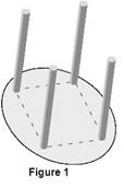
element antenna refers to an array like the one shown in Figure 1. Elements are
¼l in length, the size of the square may vary for each design
but is always less than
l/2. The
frequency for the TCAS receiver is 1090 MHz, so the wavelength l is 10.83”.
The four
element antenna is used by both Honeywell and Collins for intruder bearing
detection in their phase TCAS systems. The
physics behind this detection principle is depicted in the following figure:
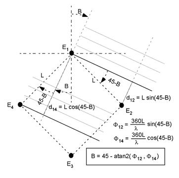
Figure 2.
The phases in the above equations would be the ones that
would be measured in opened elements, or in other words, in the unrealistic
absence of currents. Yet, some energy needs to be absorbed from the incident
wave to feed the receiver input circuits, so there will definitely be current in
every element. These reactive currents will induce voltages in the neighboring
elements affecting the phases to be measured. Fortunately, symmetry forces any
reactive phase shift in F43 to
be the same as in F12 and
also forces shifts in F23 to
be the same as in F14, So, as
for canceling out the mentioned reactive effects of a real antenna, the sum of
these phase shifts is introduced in the above expression for the bearing.
B = 45 – atan2(F12 + F43 , F14 + F23)
1
If we change the references so as to keep the numbering
order we get:
B = 45 – atan2(F12 - F34 , F23 - F41)
2
Also the above can be expressed as:
B = atan2(F23 - F41, F12 - F34)
- 45
3
It may be shocking that the expression for the bearing B
is not dependent on the actual size of the antenna, yet it is not that just any
size would the same; small antennas render smaller phase shifts for the same
bearings. In other words, smaller antennas are less sensitive to intruder
bearings changes than bigger ones. Let’s do some error propagation.
Allow Q to be the quotient in the inverse tangent
Q = Y/X = (F23 - F41)/(F12 - F34)
4
Differentiating the quotient
dQ = dY/X –
YdX/X2 = (Y/X)(dY/Y – dX/X) = Q(dX/X - dY/Y)
5
The increments absolute values dX and dY may be taken as
the unwanted RF path differences, while Y and X, are the phase spans. The signs
of the unwanted differences must be assumed to render the worse case
calculation, so let:
dQ = 2Q dA/A
6
Now, differentiating the inverse tangent respect to Q:
dB = (180/p) dQ/(1 +Q2)
7
dB = (180/p) (dA/A) 2Q/(1 +Q2)
The function 2Q/(1+ Q2) has a maximum of 1 for
Q=1; the maximum for dB must then be:
dB = (180/p) (dA/A)
8
The maximum acceptable path error for a specified bearing
tolerance dB is:
dA = dB
A/(180/p)o
9
Say L = 3.8",since l = 1084" at 1090 MHz, then the maximum phase shift or phase span would be 126°. If dB was to be specified to less than 10°, being A equal to its phase span of 126°, equation 9 would render that the maximum path error that could be tolerated is 22°,which would allow about half an inch error in the coaxial cabling lengths while in operation. A smaller antenna, say one with L = 2.65", would feature a phase span of only 88°. If a 3° accuracy is specified the path tolerance would only be 0.1". In this case, even small temperature gradients during flight may amount to these differences in thermal expansion, so periodic recalibration would be necessary.
A
perfectly loaded dipole absorbs power from an incident electro-magnetic wave,
leaving a shadow behind it. Though
this shadowing effect practically disappears due to diffraction after a few wave
lengths, a dipole within a shadow will be absorbing less power from the wave.
The amplitudes of the received signals in quad dipole antenna will then depend
on the wave angle of incidence, since the dipoles in the back will be shadowed
more or less depending on how behind they are to the front ones. TCAS amplitude
systems take advantage of this effect allowing their bearing determinations to
challenge in accuracy those of phase systems.
For
estimating just how much attenuation could be involved in this effect the front
dipole may be simplified a perfectly opaque object with an area equal its
effective area Aeff.
Aeff = G l2 /4p
1
Where G,
is the Gain or directivity of the antenna that for the Hertzian dipole is 3/2.
Considering this area to be shaped as a rectangle with a length equal to that of
the half wave dipole, we get the following expression for it width W:
W = Aeff /(l /2) = 3l /4p
2
Going
now to the problem of the edge diffraction, consider a path profile model for
the single knife edge diffraction*.
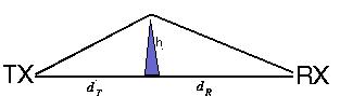
Figure 3
If the
direct line-of-sight is obstructed by a single knife-edge type of obstacle, with
height h we
define the following diffraction parameter v:
v = h Ö((2/l)(1/dr+1/dR)
3
Where dt and dR are
the terminal distances from the knife edge. The diffraction loss, expressed in
dB, can be closely approximated by
AD=0
if v <
0
4
AD=6 + 9 v +
1.27 v2
if 0 < v <
2.4
5
AD=13 + 20 log v
if v >2.4
6
The
attenuation over rounded obstacles is usually higher than AD in
the above formulas. Since our object is not a sharp one, the actual attenuations
can be expected to be greater that the calculations.
Since we
are dealing with plane, waves the distance to the transmitter can be regarded as
infinite; let dR be
equal to ¼ l, which is about the size L in the antennas; finally, let h be
equal to ½W:
v = ½WÖ((2/l)(1/(¼ l)) = (W/l)Ö2= 3/(2pÖ2) = 1.06
7
Substituting in equation 5:
AD = 16.97 dB
8
At this
point, we can conclude that the attenuation when a dipole is directly behind
another should be greater than 15 dB. This would be the case for E3 and E4 (see
Figure1) with a wave incident at 45°. Ratio for E1 and E2 will
be of 0 dB. For an incidence of 0°, attenuation for E2 and E4,
will be the same and not much below E1,
since they should be almost out or completely of the shade, depending on the
size of the antenna. E3 will
be showing the greatest attenuation for being directly behind E1.
In the octant from 0° to
45° E4 will
change from near 0 dB attenuation to more than 15 dB. For
smoothly covering the octant, the length of the diagonal should be equal to or
slightly less than W.
*http://www.wirelesscommunication.nl/reference/chaptr03/diffrac.htm