About Signal Spectrum
The spectrum of a signal is defined as its Fourier Transform, the mathematical expression of which is:
![]()
![]()
Where f(w) is said to be the spectrum of the signal g(t). In practice, no signal function is known from -¥ to ¥, but only in a limited time interval. So, an assumption must be made for the unknown part of the time.
There are two common assumptions:
The first renders the “line” spectrum of all periodic signals in which the power
concentrates at frequencies that are multiple of 1/T, where T is the time
interval involved. Said in other words, the Fourier integral becomes a Fourier s
Let’s consider the following wave form and assume it repeats itself after time T:
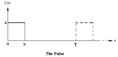
Figure 1
The power spectrum of the above signal with the repetition assumption is:
Figure 2
As T is increased to infinite (approaching the second assumption) 1/T tends to zero; the lines become closer and closer until, in the limit, the spectrum becomes continuous (Figure 3). Of course, also the power of each the lines go to zero, that's why we changed vertical axis from power to power density (power per frequency unit).
Figure 3
Modern Spectrum Analyzers digitize the signals and use the FFT for delivering the spectrum, the old school uses analog approaches, the most common of which is that of mixing the signal with a local oscillator; then sweeping its frequency and displaying the output of a narrow bandwidth amplifier, called the IF (Intermediate Frequency) amplifier. What we are about to discuss affects the measurement of a spectrum no matter what method is used.
There is no way to measure the continuous spectrum of a single event, like that of the single pulse discussed above, because this would always involve some sort of infinite.
For the analog spectrum analyzer, the pulse must repeat so that it can mix many times with the sweeping frequency of the local oscillator rendering, this way, enough hits for the spectrum shape to show.
The digital approach seems to accomplish that goal because a single pulse can be digitized. Yet, only a finite number of samples can be taken, rendering only a finite number of frequency points in the FFT spectrum. That is perfectly equivalent to the “line” spectrum of a repeating pulse.
Another case that seems to defy the assertion that a continuous spectrum cannot be measured is that of the noise spectrum. A spectrum analyzer seems to render a continuous spectrum in a single sweep. The problem here is that every sweep renders a slightly different result. No matter if you average or slow down the sweep, obtaining the exact spectrum will involve infinite time.
Assume that a perfect sine wave is available for measurement, yet an analog spectrum analyzer will always show a bell shaped spectrum and not a sharp line. That explains easy enough, what you are looking at is the frequency response of its IF amplifier. If we made its band narrower, the bell should sharpen, right? That’s true, but it happens that, at the same sweep rate, the power of the peak will seem to lower and shift to the end of the sweep. The reason for this is that the time response of the IF amplifier goes inverse with its bandwidth. To avoid this, the sweep must be slowed down as the bandwidth is narrowed. In the limit, a line spectrum can only be obtained with an infinite sweep time
But this is not just a technical limitation of analog spectrum analyzers, same happens with the digital approach. A sharper spectrum requires the sampling of more sine wave periods, i.e. a longer sampling time.
So here’s what happens, you cannot know exactly the frequency composition at a specified instant, you can only know that frequencies are within a band during a time interval. The longer the interval, the more exactly frequencies can be known. The bandwidth Dw and the interval Dt are bounded by the following inequation.
Dw * Dt
> K
For the above to express anything beyond the mere concept, precise definitions of bandwidths and time intervals are required. Actually, rigorous statements of this principle involve second order moments of f(w) and g(t). In practice, Dw and Dt are defined as the band or time interval within 6 dB of the power peak. Only for very specific bell shaped spectrums and waveforms this K constant can be as small as 0.315, but for all practical calculations and conceptual exercises K= 1 is good enough.
This that has just shown up regarding time waveforms and signal spectra, also shows up again in the nature of elementary particles and photons. You can’t know both the position and momentum of an electron neither it’s exact energy at a particular instant in time… this is known as the Heisenberg Uncertainty Principle of quantum mechanics
What shows on the screen of a Spectrum Analyzer, as follows from the above, is not straight forward and can easily be misunderstood. It is not unusual to hear from someone using the spectrum analyzer and saying:
When using fast sweep with slowly varying signal, it is
tempting to say such as above. Yet, the uncertainty principle does not allow
that kind of talk; instants and frequencies should not share the same sentence.
To speak about spectrum, you must always consider a time interval greater than
the inverse of the bandwidth of the spectrum you are referring to. If you are
analyzing a whole second, then you could know your spectrum only with 1 Hz
detail. If you analyzed, say 5 cycles, of a periodic signal, then you can only
know the spectrum within a band as wide as
In rigor, a spectrum cannot be a function of time since it is defined as an integral over all the time ever. Yet, you can see a time varying spectrum on the screen of a Spectrum Analyzer. What then are you looking at?
What is being displayed in that screen is what a piece of the spectrum would look like if the input waveform during the time interval of the sweep had being repeating since the “big bang” and will be kept repeating ever after. For the shape that shows on the screen to bear a significant resemblance to the mentioned piece of the spectrum, the time of the sweep has to be much greater than inverse of the frequency resolution needed. Say you are scanning 1 MHz and need to resolve, say 10 KHz, then each 1/100th of the scan will require more than 0.1 ms, so the whole scan needs to be greater than 10 ms.
Let’s consider the spectrum of a CPMFSK (Continuously Phase Modulated Frequency Shift Keyed) signal. In other words, it is a sine signal that would have a higher frequency f1 during some intervals and a lower one f2 the rest of the time. The CP part of the acronym means that the frequency transitions must be made without abrupt phase changes.
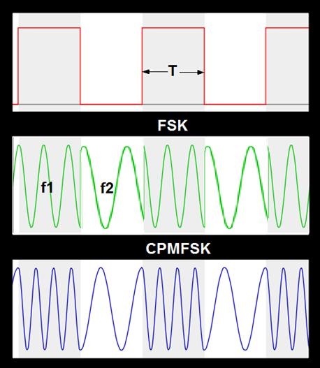
Figure 4
For simplicity, let’s consider the case in which f1 intervals T are all equal and also equal to those with f2. Frequencies in Figure 4 are:
f1 = 3.5/T
f2 = 1.5/T
The wave forms in Figure 4 can be thought as the superposition of two pulse modulated wave trains as in Figure 5:
Figure 5
The amplitude spectrum of a periodic function is, in general, a set of complex numbers, but if an origin can be found that makes the said function perfectly even (f(t)=f(-t)) or odd (f(t)=-f(-t)), then the amplitude spectrum would be a set of real (cosine series) or imaginary numbers (sine series) respectively. In this case, both components are odd from origin O, so the amplitudes of its sine series and its sum can be plotted in a simple chart as follows:
Figure 6
Couple of interesting things here:
Let’s consider now the case of a real signal, say a NRZ (No Return to Zero) bit stream. The distinction between a NRZ binary modulation and a RZ is as follows. Binary transmission require, at least, two states the On and the Off states”. For the NRZ case, the On state is plainly the One, while the Off is the Zero, period. The RZ, is the pulse/no pulse case, in other words, for a One, the signal goes to the On state for half the bit rate period and comes back to Off (Returns to Zero) for the rest. For a Zero, the signal stays in the off state for the whole bit rate period.
Again, we can split the CPMFSK signal in two amplitude modulated pulse streams components. Invoking the theorem that says that the Fourier transform of the a signal’s auto correlation function is equal to its power spectrum, it can be proved that the power spectrum for each of the said components is a continuous (sin(x)/x)2 like that of Figure 3, zeroing at every multiple of the bit rate.
Intuitively, one can get near to the above conclusion. First, why is there no power at frequencies that are multiple of the bit rate? For the answer, let’s consider the base band, this is the modulation signal only. Within the bit rate period, the signal is either Off or On, integration of a sine or cosine with a period equal to this bit rate period must render 0 for whatever the value of the signal might have. For frequencies other than these exact multiples, the integral must render some value different than 0, yet as frequency goes up, the part of the sine/cosine that does not cancel away gets smaller, so the amplitudes must die off with 1/f. So, the power spectrum in Figure 3 would have been a good guess.
We know that modulating a carrier with frequency f0 with a signal having whatever base band spectrum, will show a similarly shaped spectrum, but around f0.
Back to the CPMFSK signal, if the difference between the two frequencies being keyed, f1 and f2, is several times greater than the bit rate, then the combined power spectrum should look something like Figure 7.
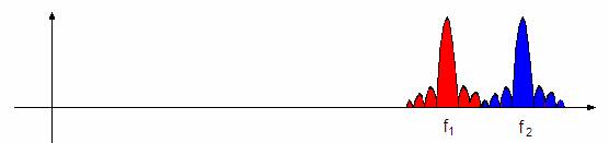
Figure 7
As the bit rate increases, the amplitude spectral components will start inferring, either by enhancement or cancellation. As we saw in the simplified example above, keeping the phase transition continuous will favor the enhancements of the spectral components within the f1-f2 interval, as well as the cancellation of those outside of it. So, for high bit rates, the spectrum for the CPMFSK modulated signal can be expected to be narrower than each of its amplitude modulated components (Figure 8), therefore the advantage of this modulation method.
Figure 8